Confidence Intervals
Why use it?
Confidence intervals help to quantify our uncertainty due to random sampling. When we take a sample from a process we use statistics to estimate the location of a population parameter. Because there is variability in these statistical estimates due to random sampling, we need to quantify our uncertainty. Confidence intervals also help us develop the concept of hypothesis testing.
What does it do?
Confidence intervals provide ranges for population parameters (e.g., averages, standard deviations, and proportions) with a certain confidence. When a given population is sampled many times, the calculated sample averages can be different even though the population is stable (as shown in the following figure). Confidence intervals quantify the uncertainty by describing how likely it is that a population parameter lies within a certain range of values. Typically we calculate 95% confidence intervals, meaning we are 95% confident that the population parameter lies within the interval. Conversely, there is a 5% risk (the alpha risk (α) = 1−Confidence = 1−0.95 = 0.05) that the population parameter does not lie within the interval.
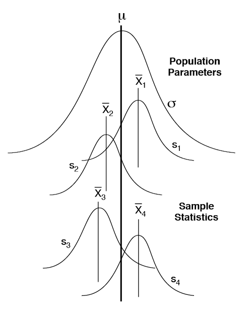
The differences in these sample averages are simply due to the nature of random sampling. Given that these differences exist, the key is to estimate the true population parameter. The confidence interval allows the organization to estimate the true population parameter with a certain confidence.
The confidence interval is bounded by a lower limit and an upper limit that are determined by the risk associated with making a wrong conclusion about the parameter of interest. For example, if the 95% confidence interval is calculated for a subgroup of data of sample size n, and the lower confidence limit and the upper confidence limit are determined to be 85.2 and 89.3, respectively, it can be stated with 95% confidence that the true population average lies between these values. Conversely, there is a 5% risk that this interval does not contain the true population average.
Note:
- When sampling from a process, the samples are assumed to be randomly chosen and the subgroups are assumed to be independent
- Whether the true population average lies within the upper and lower confidence limits cannot be known unless we measure the whole population
- It is extremely rare that we have access to measurements for the whole population. Most statistical packages assume that the data we supply come from a sample
How do I do it?
Depending on the population parameter of interest, the sample statistics that are used to calculate the confidence interval subscribe to different distributions. Aspects of these distributions are used in the calculation of the confidence intervals. Listed below are the different confidence intervals, the distribution the sample statistics subscribe to, the formulas to calculate the intervals, and an example of each. Notice how these confidence intervals are affected by the sample size, n. Larger sample sizes result in tighter confidence intervals, as expected from the Central Limit Theorem. Confidence intervals are also affected by the alpha risk. As we increase the alpha risk (from 5% to 10%, for example) the confidence interval becomes tighter.
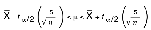
Confidence Interval for the Mean
The confidence interval for the mean utilizes a t-distribution and can be calculated using the following formula:
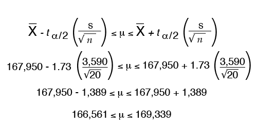
Example:
A manufacturer of inserts for an automotive engine application was interested in knowing, with 90% confidence, the average strength of the inserts currently being manufactured. A sample of 20 inserts was selected and tested on a tensile tester. The average strength and standard deviation of these samples were determined to be 167,950 and 3,590 psi, respectively. The confidence interval for the mean µ would be:
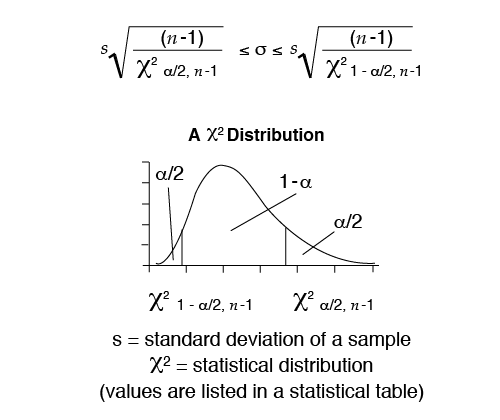
Confidence Interval for the Standard Deviation
The confidence interval for the standard deviation subscribes to a chi-square distribution and can be calculated as follows:
Example:
A manufacturer of nylon fiber is interested in knowing, with 95% confidence, the amount of variability in the tenacity (a measure of strength) of a specific yarn fiber they are producing. A sample of 14 tubes of yarn was collected, and the average tenacity and standard deviation were determined to be 2.830 and 0.341 g/denier, respectively. To calculate the 95% confidence interval for the standard deviation:
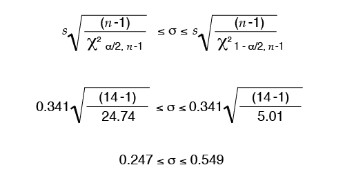
Caution: Some software and texts will reverse the direction of reading the table; therefore, χ2α/2, n -1 would be 5.01, not 24.74.
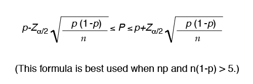
Confidence Interval for the Proportion Defective
The exact solution for proportion defective (p) utilizes the binomial distribution; however, in this example the normal approximation will be used. The normal approximation to the binomial may be used when np and n(1-p) are greater than or equal to five. A statistical software package will use the binomial distribution.